Wednesday, September 5, 2012

PHOTOGRAMMETRY FOR THE SURVEYOR

1. General

For many years I have attempted to provide my clientele with the best service possible. More learned scholars and I have differed in my general approach over the years. One simple premise which is undeniable: "follow in the footsteps of the original surveyor". Many times this premise is extremely difficult and time consuming. At best, the opinion may not have a high degree of certainty. We as surveyors do not have to achieve "beyond a shadow of doubt" and can rely on a "preponderance of evidence".

Furthermore, our task is not to merely define the present evidence, but to ascertain "a snapshot in time" for those conditions predominate as of the date of the conveyance description. The conveyance date is not attributable to the last deed of record, but that date of the original scrivener. A difficult task. Often the description presented has been utilized or 50 years, from owner to owner and thus perpetuating the title. We then must rely on what I term "my way-back machine". Does our commission constitute the first actual survey? What were those conditions at the time of the original conveyance?

Reliance on aerial photography is a time honored procedure; but unfortunately only qualitative information is readily available. Techniques derived 100 years ago can enhance the data available through stereo modeling. Many of the commercial programs are beyond the financial reach of the average surveyor and the public domain programs (i.e. GRASS, et. al.) are time consuming to learn.

Deed calls that have never been surveyed, and many that have, call for "to the fence line", "to the centerline of the road", "to the creek" and "to the corner of Smith’s barn". Many of us ignore this distinction as superfluous. Not correct. The point called for may not presently exist. We must first extinguish our resources before accepting the default. Examples of this need are redundant and I am sure you can devise your own if you are reading this. As this investigation proceeds, I will supply my own for sample problems.

Finally, source must be ascertained for stereo pairs. You may have your own and I can recommend others (later in the investigation). Also note my terminology will not be found in any textbook, because they are not consistent.

And one source I have been using is
cartlab@bama.ua.edu . About 10,000ft but is a scan of the print. Available from 1955 to 2009. Most stereo pairs. About 30Mb each 9" contact print.

Also, http://www.usgs.gov/pubprod/aerial.html High altitude = 40,000 BUT includes camera data. Average file 1Gb.
I think if we combine all our resources we can identify many unknown storage locations that will benefit all.
2. Brief Theory, Standard Conditions and Chronology


As time has permitted, I have tried to develop my own system, albeit somewhat clumsy and hopefully you can benefit from my long and tedious study. The theory is divided into two distinct observations 1) internal conditions and 2) external conditions. The internal characteristics must be solved first so we will discuss these calculations first. Figure below shows the basic internal set of parameters. The aircraft is flying along the "Y" axis at some angle oriented from the global coordinate system. The lense center is termed the exposure station and the orthogonal distance from the lense center to the film is termed the focal length. For a vertical photograph scale is easily determined and for level terrain measurements can be made from the positive. However, very rarely is the photograph truly vertical and tilt, yaw and roll values of 1 to 3 degrees are not uncommon. To the layman, the photograph appears as a true orthographic projection of the earths surface.


Not so, Dr. Watson, it is a perspective projection and the rules of perspective geometry apply. The intent of this treatise can not be construed to fully explain the mathematics and principles required to determine the unknown parameters. The fundamentals will be presented, similar to a plain surveying course and reading materials for your own investigation.

An example aerial photograph, recently utilized for one of my projects, is shown as Figure "147 Cropped". This photo is one of a stereo pair dated 1964 in Cullman County at Berlin Crossroads on US 278.
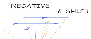
The middle fiducial mark is shown in the upper left corner and below a race track at the upper middle, no longer in place. Note that at the intersection of the county road south of US 278, the county road appears to have a curvature to the west. Actually the centerline is a straight line and a good example of relief displacement. The section line is shown immediately south of the #014043. The photo is oriented generally north. Thus the point here is relief displacement and its effect to our investigation(s). I have provided a figure which describes this parameter. This figure shows the delta change in the negative due to a vertical change in elevation. The negative position is in Region I, whereas the positive is Region III, trigonometrically. This is only one parameter that must be accounted for.

Remember, the discussion is presently directed for the internal characteristics of the individual photograph. The details shown are for level flight for convenience. We must make similar adjustments for non level flight, altitude and camera. The change in analysis of an individual photograph today is significantly different from those procedures I utilized as a young engineer and surveyor. Desktop computing has revolutionized data acquisition. The complex and expensive stereoplotter of yesterday is no longer necessary and this aspect encouraged the writer to pursue an economical means to utilize historical aerial photography. For a survey purposes, data acquisition is normally limited to one stereo model; whereas, photogrammetrists deal with entire counties and entail thousands of models.

Nearly ten years ago, pursuant to environmental investigations, I discovered the availability of various photography from the US government agencies and historical organizations, many dating to the 1950's. Often in my career I have wished to be able to ascertain the location of a specific topographic detail pertinent to the deed furnished. Thus I began a ten year quest that consisted of available textbooks, CEU courses and languages i.e., Visual Basic, C++ and FORTRAN compilers. Further any public domain software that would assist my limited knowledge with the matrix manipulations and least squares estimations were ferreted out.


3. Church’s Method and the Collinearity Equations
 
By chance I found Dr. Church’s "ELEMENTS OF PHOTOGRAMMETRY", 1948 Enhanced Edition, through one of AMAZON.com’s affiliates. Dr. Church and Dr. Quinn state in the preface "This book has been prepared to serve as a textbook for an introductory course in elementary photogrammetry. This edition presents the history and background of photogrammetry together with the basic principles and fundamental applications now possible in this most fascinating field". They further state on page 57 "A very important feature of this problem, however, is that it provides a means of measuring parallaxes without a stereoscope, linear measurements with an engineers scale being sufficient for finding the line of flight....This makes possible all of the photogrammetric operations...without the use of any equipment other than the photographs themselves and an ordinary engineer’s scale". Dr Church provided his expertise to the WW II war effort and afterwards at Syracuse University and The ASPRS for many years.

A straight line is a straight line. From Wolf, Elementary Photogrammetry , Second Edition, pg 245:

The method of space resection by collinearity is a purely numerical method that simultaneously yields all six elements of exterior orientation. Normally the angular values of omega, phi, and kappa are obtained in the solution..... Space resection by collinearity permits the use of redundant amounts of ground control; hence least squares computational techniques can be used to determine most probable values for the six elements. The procedure, although computationally lengthy, is readily programmed for computer solution so that the calculations are routinely performed. Space resection by collinearity is the preferred method of determining the elements of exterior orientation.
Space resection by collinearity involves formulating the so-called collinearity equations for a number of control points whose X, Y, and Z ground coordinates are known and whose images appear in the tilted photo. The equations are then solved for the six unknown elements of exterior orientation which appear in them. The collinearity equations express the condition that for any given photograph the exposure station, any object point and its corresponding image all lie on a straight line.

The solution can be a single ray oriented whereas you minimize the residuals for a single line to a control point. Otherwise you can minimize the entire system of lines involved utilizing all control points simultaneously. Believe me the statement "is readily programmed for solution" is an understatement. Maybe for them. Be advised, the mathematics is not for the faint of heart. 


Tuesday, April 17, 2012

Photogrammetry Details


One of the aspects not mentioned in the "Turning Points" description is the relative costs of photogrammetric rectification packages. I found them from $1000, most at $5000 and many to $25,000. As stated the public domain packages are time intensive to acquire sufficient expertise to utilize efficiently.


Shown here are the first two(2) figures.


This is Photo 147 cropped showing Highway 278 at Berlin

RESOLVING THE INTERNAL PHOTO RELATIONSHIPS
begin program output:
6
 11.836        76.037        152.4         669834.458    463903.566    256.253
-68.496        65.061        152.4         668211.814    463681.834    250.363
-19.952       -79.102        152.4         669225.487    460785.233    234.913
 68.597       -97.614        152.4         670994.677    460440.17     230.545
-70.431       -4.206         152.4         668181.048    462277.202    231.57
 56.594        4.138         152.4         670742.478    462467.424    243.797

 0             0             0             0             0             5000
*********** end of Input file ************************************************
omega =        0             phi =         0            kappa =        0
XL =           0             YL =          0             ZL =          5000
****************** BEGIN ITERATION ONE ***************************************

Comment: There will be 10 iterations, one pass for each control point--------------------------------------------------
Rotation matrix for Iteration:             1
 1             0             0
 0             1             0
 0             0             1
Rotation Matrix Check
 1             0             0
 0             1             0
 0             0             1
Pt Number      1
formulating b matrix
linerarized Collinearity condition for current parameters
vxa =         -21507.6024100164
vya =         -14827.5620870508
xa1 =          21519.4384100164
ya1 =          14903.5990870508
 11.8359999999993
 76.0370000000003
Pt Number      2
formulating b matrix
linerarized Collinearity condition for current parameters
vxa =         -21509.1830364198
vya =         -14812.9415719018
xa1 =          21440.6870364198
ya1 =          14878.0025719018
-68.4959999999992
 65.0609999999979
Pt Number      3
formulating b matrix
linerarized Collinearity condition for current parameters
vxa =         -21423.5411094538
vya =         -14816.2242202659
xa1 =          21403.5891094538
ya1 =          14737.1222202659
-19.9520000000011
-79.101999999999
Pt Number      4
formulating b matrix
linerarized Collinearity condition for current parameters
vxa =         -21371.9216283967
vya =         -14810.2136383235
xa1 =          21440.5186283967
ya1 =          14712.5996383235
 68.5969999999979
-97.6139999999996
Pt Number      5
formulating b matrix
linerarized Collinearity condition for current parameters
vxa =         -21425.6342252125
vya =         -14778.6801109338
xa1 =          21355.2032252125
ya1 =          14774.4741109338
-70.4310000000005
-4.20600000000013
Pt Number      6
formulating b matrix
linerarized Collinearity condition for current parameters
vxa =         -21435.5823531119
vya =         -14814.4127257785
xa1 =          21492.1763531119
ya1 =          14818.5507257785
 56.594000000001
 4.13800000000083
---------------------
array VectorOut, sub Solve()
 82152821.8583712
-119136061.605371
-426201.315633722
-6966.59328362713
-2845.77156829018
 208.883605432399
 0
 0
 0
 0
---------------------
Sub gaussj
residuals for iteration      1
-0.01013194865169 -1.30050869153706E-02 -8.68642904038754E-03 -673688.904051919  217178.576640219 -2329.78383791447 
omega =        0.01013194865169            phi =         1.30050869153706E-02       kappa =        8.68642904038754E-03
XL =           673688.904051919            YL =         -217178.576640219            ZL =          7329.78383791447

Comment: This is the end of iteration 1,  shown are the residuals----------------------------------
Comment: There are 8 iterations similar to the above.
Comment: Begin the last iteration:
---------------------
Rotation matrix for Iteration:             10
 0.999878738904567           8.73254449169687E-03       -1.28938029034804E-02
-8.60001326212023E-03        0.999909985332769           1.02985923170277E-02
 0.012982575187713          -1.01864566224728E-02        0.999863835151054
Rotation Matrix Check
 0.999878738904567           8.73254449169687E-03       -1.28938029034804E-02
-8.60001326212023E-03        0.999909985332769           1.02985923170277E-02
 0.012982575187713          -1.01864566224728E-02        0.999863835151054
Pt Number      1
formulating b matrix
linerarized Collinearity condition for current parameters
vxa =          0.043210130460256
vya =          6.03101648868778E-02
xa1 =          11.7927898707966
ya1 =          75.9766895748996
 11.8360000012569
 76.0369997397865
Pt Number      2
formulating b matrix
linerarized Collinearity condition for current parameters
vxa =         -3.40662949737127E-03
vya =         -0.048007763032459
xa1 =         -68.4925933702779
ya1 =          65.1090075062389
-68.4959999997752
 65.0609997432065
Pt Number      3
formulating b matrix
linerarized Collinearity condition for current parameters
vxa =         -8.35992118613723E-02
vya =         -8.55772187611816E-02
xa1 =         -19.8684007895645
ya1 =         -79.0164230437273
-19.9520000014258
-79.1020002624885
Pt Number      4
formulating b matrix
linerarized Collinearity condition for current parameters
vxa =          6.81194962058081E-03
vya =          5.40036079379968E-02
xa1 =          68.5901880507898
ya1 =         -97.6680038737459
 68.5970000004104
-97.6140002658079
Pt Number      5
formulating b matrix
linerarized Collinearity condition for current parameters
vxa =          0.062432048006606
vya =          1.43609441158232E-02
xa1 =         -70.4934320492948
ya1 =         -4.22036120131746
-70.4310000012882
-4.20600025720164
Pt Number      6
formulating b matrix
linerarized Collinearity condition for current parameters
vxa =         -2.52434608293936E-02
vya =          4.2791432117453E-03
xa1 =          56.6192434617323
ya1 =          4.13372059434486
 56.5940000009029
 4.1379997375566
---------------------
array VectorOut, sub Solve()
-3.9193457756315E-06
-2.27558512645529E-07
 6.38136271862301E-08
-1.07887282052499E-09
-1.07936164293905E-09
 3.75699982703177E-11
 0
 0
 0
 0
---------------------
Sub gaussj
residuals for iteration      10

Comment: The following are the residuals for -10-.... notice values are small.
-6.58650037074729E-14 -1.05427665029161E-13 -1.77141193660531E-13  2.74643877656817E-10 -7.27011384398665E-08 -3.99021923776564E-11

Comment: Then, finally the 3 rotations and the coordinates of the Observation Point. Also in the actual output file, an ASCII file, these values will be on one line.
  Final Values: omega   phi  kappa XL  YL  ZL -------------------------
 1.01874913978596E-02        1.29829399116193E-02        8.60084414823962E-03        669650.413992352            462343.808977171            3305.40699175135
degrees
 0.583700260923186           0.743867662607736           0.492792069943922

Comment: End of Output File.
After the internal characteristics are determined for both photos, omega phi kappa XL YL ZL, we can then utilized those photo relationships to establish an unknown ground point.

At this milestone of the process, the redundant input can "shroud" a poor control point (or the photo coordinates), just as a single measurement can be hidden for a survey that has 100 observations. Just one can have high residuals and since the remainder have small residuals they "overwhelm" to poor point.
Shown is the stereo pair, the right photo has all rotation angles = 0. Notice the difference in ground coverage. Of course all parameters are exaggerated for clarity of the viewer.
Figure showing an unknown ground point and the ray intersection with both photo positives.


These are the OP values w/o adjustment for earth curvature: 

Final Values: omega   phi  kappa XL  YL  ZL -------------------------
 1.01874913978596E-02        1.29829399116193E-02        8.60084414823962E-03       

      XL 669650.41                  YL 462343.81           Z 3305.41
degrees
 0.583700260923186           0.743867662607736           0.492792069943922


These values are final OP with curvature adjustments:

 Final Values: omega   phi  kappa XL  YL  ZL -------------------------
 8.87707101416532E-03        1.35039640397676E-02        9.21384170508731E-03       

     XL  669652.98                  YL  462349.56            Z  3306.65
degrees
 0.50861870354959            0.773720146175117           0.527914242803126


The phi & kappa rotations show some variations.

data concerning atmospheric refraction:
See Analytic Aerotriangulation, 1962 Coast And Geodetic Survey, Technical Bulletin No 21, Dated July 1963
He states an average terrain height can assumed over the area involved.  The K coefficient is dependent upon the barometric pressure and the wavelength of light and other parameters. These can be simplified for the project area; thus for our applications we can normally assume both flight paths are completed in the same day. Paul Wolf also has a slightly different approach.
Harris, 1962.
                                                                              
Also note here that Harris used f = c, so the focal length "f" is the parameter "c" in the equation.


So here we see the external conditions being evaluated using the collinearity equations for two lines.


Wolf states:
"These are the two equations for a straight line in an image, corresponding to the two collinearity equations for a point in an image. The photogrammetric condition equations using straight lines will fail when the straight line in object space is in the same plane as the two (or more) image perspective centers (the epipolar condition). When this occurs, the projection planes for the corresponding straight lines from the images are coplanar. Since the planes do not intersect in a single line, the object line cannot be  determined, Consequently, in practice, straight lines that are parallel or are close to parallel to the epipolar plane should be avoided. "

Sample input for the solution of the unknown value. This routine is yet to be finished. The image adjustments are made from a spreadsheet:

9652.79465192302            2349.70930221402            3306.963    8.8332392387544E-03         1.34473361198426E-02        9.21546910637473E-03  152.4
9673.07190937109            4018.56307591905            3307.66     8.04394743779159E-03        8.42477365500256E-03        0.013275825020702     152.4
3
 56.6068          4.017     53.709       -79.604     10742.478     2467.424      0
  64.3287      50.4046    61.6548      -33.0248   10838           4634         235
  64.1585      49.7376    61.4927      -33.6192   10838           4634         235


For the above: You must have  an estimated value for the unknown point so that GAUSS will know where to start, i.e. 10838  4634  235.
Some Output:

Estimated point coordinates and iteration deltas, Iteration 1
XL :  10742.575       0.097 YL :   2467.669       0.245 ZL :    261.430     261.430
Image Errors Left   Photo   4.085     0.405          Right      3.801    -5.763

...........................................
Estimated Point coordinates and iteration deltas, Iteration 10
XL :  10742.574       0.000 YL :   2467.652      -0.000 ZL :    242.167      -0.000
Image Errors Left  Photo   0.074    -0.001         Right    -0.074     0.002


How would you check yourself?
Include a point, say #1 of the 3 above that has a known elevation and position. Or say one that has a known elevation. Very prudent issue.
Add to bibliography shown in "Turning Points":

9)Sprott, Julien, Numerical Recipes Routines and Examples in BASIC, Cambridge University Press, 1998

10) Press, William Et Al., Numerical Recipes in Fortran 77, Cambridge University Press, 2003

All contents Copyright 2012, J M Hillman